Decision Trees and Random Forests

Prof. Forrest Davis

Apply a decision tree to new data

• Consider the following decision tree (from the book).

Question: Classify a new data point with the following values:

• petal length: 2.50cm
• petal width: 1.75cm

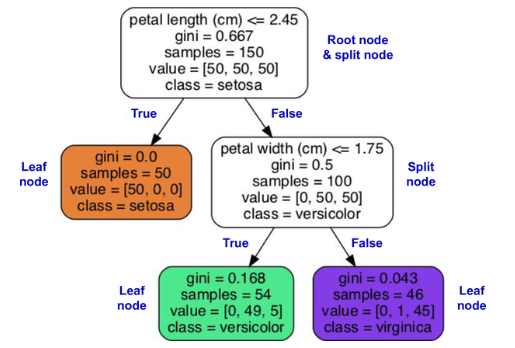
Answer: The point would be classified as veriscolor

Step One: A classification problem (our old friend, the bad plots)

• Consider the following figure.

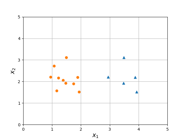
Question: Calculate the Gini impurity.

• Hint: You can get the Gini impurity if you can answer the following question:

  • What is the probability of classifying a point incorrectly (e.g., if I select a triangle, and I guessed based on the labels I know exist, what is the likelihood I misclassify a triangle)?

Answer

• Starting with the triangle class that I mispredict as circle

\begin{align} G_\textrm{triangle} &= P(\textrm{select triangle}) * (1 - P(\textrm{classify as triangle}))\\ &= \frac{5}{15} * (1-\frac{5}{15}) \\ &= \frac{2}{9} \end{align}

• Next up with the circle class that I mispredict as a triangle

\begin{align} G_\textrm{circle} &= P(\textrm{circle}) * (1 - P(\textrm{classify as circle}))\\ &= \frac{10}{15} * (1-\frac{10}{15}) \\ &= \frac{2}{9} \end{align}

• Total probability of misclassification is $\frac{4}{9} \approx 0.44$
• Notice it is less than $0.5$ why is that?

A note on the equation

• Above we use $G_\textrm{i} = \sum_{k=1}^n P_{i,k} (1 - P_{i,k})$ where $n$ is the number of output classes and $P_{i,k}$ is the probability of correctly guessing output $k$ (from the $n$ classes) at a node $i$ in the tree. Recall a node has some split of the data.
• The book instead uses $G_\textrm{i} = 1 - \sum_{k=1}^n P_{i,k}^2$
• These are equivalent:

\begin{align} G_\textrm{i} &= \sum_{k=1}^n P_{i,k} (1 - P_{i,k})\\ &= \sum_{k=1}^n P_{i,k} - P_{i,k}^2 \\ &= \sum_{k=1}^n P_{i,k} - \sum_{k=1}^n P_{i,k}^2 \\ &= 1 - \sum_{k=1}^n P_{i,k}^2 \\ \end{align}

Note $\sum_{k=1}^n P_{i,k}$ is 1 because, by fundmental assumption about probability, the total probability at a node $i$ for all of the classes must sum to 1.

Step Two: Apply Gini impurity

• Consider the following two potential decision boundaries:

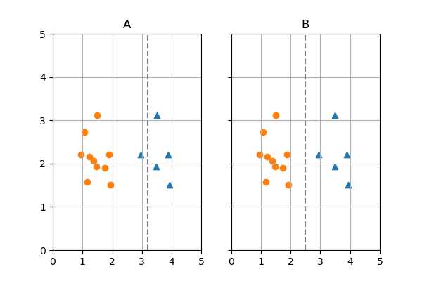
Question: Calculate the Gini impurity for the left and right regions for each decision boundary

Answer:

• Equation for Gini impurity

$$ G = 1 - \sum_{k=1}^K p_{k} ^2 $$

• Where we have $K$ output classes

• Let's start with A

• The left side has a gini index of:

$$ G_\textrm{left A} = 1 - ((\frac{10}{11})^2 + (\frac{1}{11})^2) = 0.165 $$

• The right side has a gini index of:

$$ G_\textrm{right A} = 1 - ((\frac{0}{4})^2 + (\frac{4}{4})^2) = 0 $$

• Next with B

• The left side has a gini index of:

$$ G_\textrm{left B} = 1 - ((\frac{10}{10})^2 + (\frac{0}{10})^2) = 0 $$

• The right side has a gini index of:

$$ G_\textrm{right B} = 1 - ((\frac{0}{5})^2 + (\frac{5}{5})^2) = 0 $$

Question: Calculate the CART cost function value for both decision boundaries

Answer

• The cost function is as follows:

$$\textrm{Cost}_\textrm{threshold} = \frac{m_\textrm{left}}{m}G_\textrm{left} + \frac{m_\textrm{right}}{m}G_\textrm{right}$$

• Where m is my total samples considered for this split and $G$ is gini impurity

• For A

$$ \textrm{Cost}_\textrm{A} = \frac{11}{15} * 0.165 + \frac{4}{15}*0 = 0.121$$

• For B

$$ \textrm{Cost}_\textrm{A} = \frac{10}{15} * 0 + \frac{5}{15}*0 = 0$$

Question: How much information did I gain with each decision bounday?

Answer

• For A:
  • $0.44 - 0.121 = 0.319$
• For B:
  • $0.44 - 0 = 0.44$
• I gained the most information with B, so it wins!

• Consider a binary classification task. Three decision boundaries with the following properties are generated. Determine their Gini values.

  • All points belong to class 1
  • Half of the points belong to class 1
  • None of the points belong to class 1

Step Three: CART Algorithm Sketch

Guiding Questions:

• Sketch out the CART Algorithm
• Why is this algorithm greedy?
• What are possible stopping criteria?

Answers

1. Calculate the Gini impurity for the entire dataset (e.g., impurity of the root node).
2. For each input feature, calculate the Ginit impurity for all possible thresholds. The feature, threshold pair which has the minimum Gini impurity wins.
3. Split the data based on the chosen feature, threshold pair. Create new nodes.
4. Repeate 2 and 3, until some stopping criterai is met. Could be maximum tree depth, minimum data points in a leaf node, or a minimum reduction in impurity

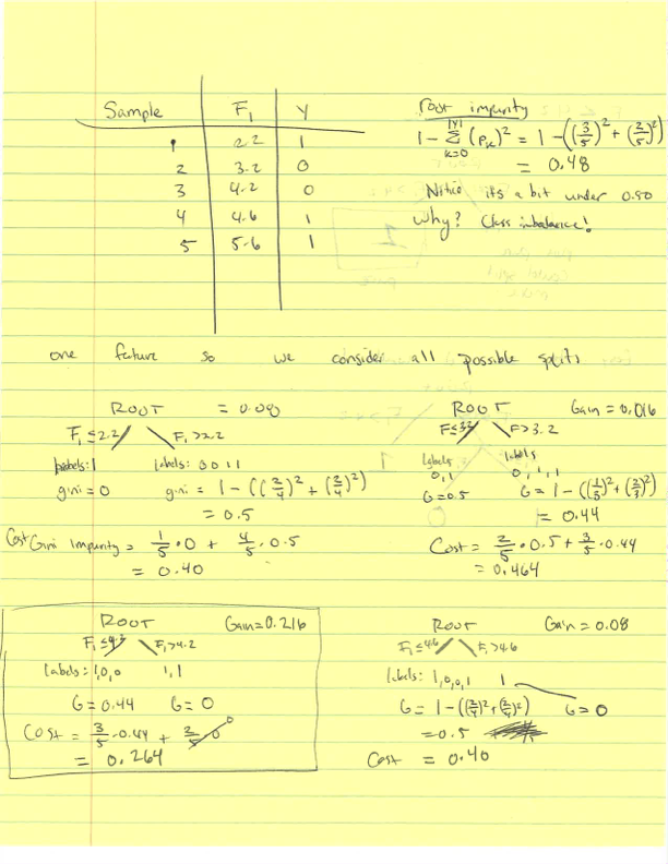
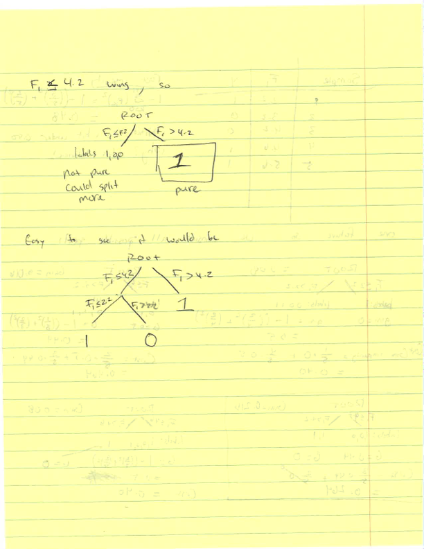
Learning a decision tree for continuous data

• Given the following sample data, use the CART algorithm to learn a decision tree.

Sample	F$_1$	Y
1	2.2	1
2	3.2	0
3	4.2	0
4	4.6	1
5	5.6	1

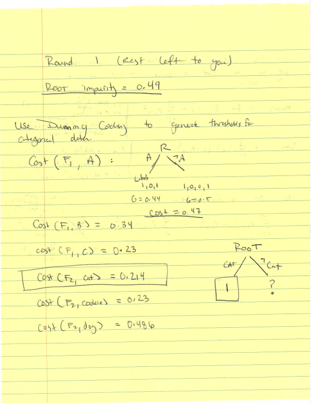
Learning a decision tree for non-binary categorical data

Question

• Given the following sample data, use the CART algorithm to learn a decision tree.

Sample	F$_1$	F$_2$	Y
1	A	cat	1
2	B	cat	1
3	A	cookie	0
4	C	cookie	0
5	C	dog	0
6	B	dog	1
7	A	cat	1

Limitations of Decision Trees

Question What are some limitations of decision trees?

Answer

• Our learning algorithm can proceed until all nodes are pure. Meaning, we can greatly overfit our data.

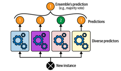
Random Forests, Ensemble Learning, and Voting Classifiers

• Random forests: train a bunch of decision trees on your data (adding in some randomness to ensure differences between each decision tree).
• Ensemble learning: train a bunch of models and use them all to make a prediction
• Voting Classifiers is one approach to ensemble learning.