Linear Regression I

COSC 410: Applied Machine Learning

Prof. Forrest Davis

Overview

• Model
  • Basic articulation
  • Mathematical tools
• Cost/Loss
  • Goals
  • Options
• Optimization/Learning
  • Goals
  • Closed form
  • Stochastic gradient descent

Model

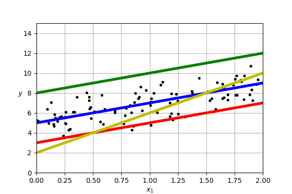
• Let's start with some fake data.
• At its core, the aim of regression is to predict a numerical value drawn from some continuous distribution

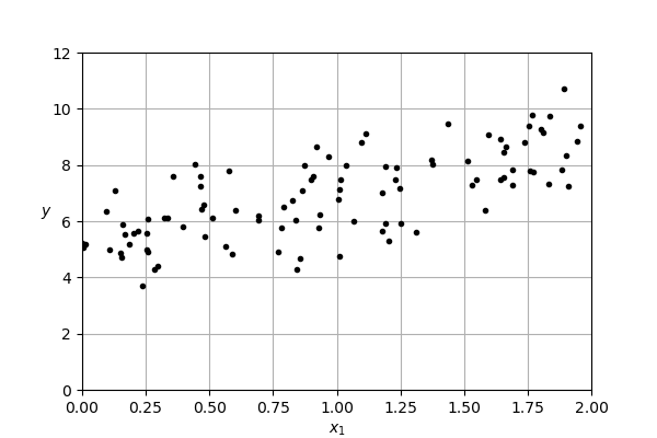
• We want to uncover the relationship between $x_1$, and $y$
• Our beginning assumption: the relationship is linear

Single point (singly none)

• Let's start with a single point, highlighted in red

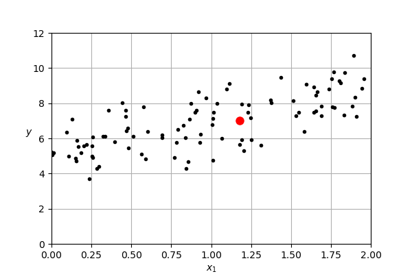
• Introducing some notation, we will refer to his point at $x^{(1)}$

  • The superscript refers to the sample
  • The subscript refers to a dimension of the input
  • E.g., $x_3^{(8)}$ refers to the 3rd dimension of the 8th input

• We are trying to find parameters that let's us predict the observed $y$ value from the input

• In this case, we want to find parameters that maps from 1.18 (our sample's first feature value) to 7

• In other words, we are trying to solve for $w_1$ in the following equation

  $$ y = w_1 x_1 + b $$

• That is, we are assuming the output is determined by a scaling of our input plus a term, which we call the bias

Question: What values would you put for $w_1$ and $b$ and why?

Answer:

$$ 7 = 1.18 w_1 + b$$

• Let's try to get the largest $w_1$ whole number we can so $5$

• $b$ is the remaining so $-1.1$

• This assume quite a large slope which we don't seem to see

• What if we assume the $w_1$ is smaller, say $2$, then $b$ would be $4.64$ (which seems to more closely accord with the distribution of the data)

• The point (no pun intended) is we can't tell with a single point. We need to sample more data to get a better sense of the underlying relationship.

Many samples (many stones can form a line)

• In considering many single dimensional samples, we need to add a mathematical object to our skill set, vectors
• A vector is an array of scalars, for example,

$$ \mathbf{a} = \left[\begin{array}{c} a_0 \\ a_1 \\ a_2 \\ \end{array}\right] $$

• $ \mathbf{a} $ is a 3 dimensional vector (i.e. $ \mathbf{a} \in \mathbb{R}^3$)

• Note: math indexes from zero, but in CS we index from 0

• Suppose we considered all our points, we would have two vectors:

  • x and y
  • We will use lowercased bold letters for vectors

• Then we are working with

$\mathbf{y} = w_1 \mathbf{x} + b$

• We can try out some different parameters and see which is better
• We are comparing our model's predictions, which we call $\mathbf{\hat{y}}$ (pronounced, y hat), to our true outputs, $\mathbf{y}$ (sometimes called gold outputs)

Many dimensions

• What if our input is composed of more than one feature (e.g., houses represented by number of rooms, number of bathrooms, square footage, etc.)?

• We'd then want to learn a weight (or parameter) for each input feature:

  $$ y = w_1 x_1 + w_2 x_2 + w_3 x_3 + ... + w_n x_n + b $$

• Notice that we have a number of scalar parameters and a number of scalar input features

• Perhaps, we can write this with reference to two vectors, $\mathbf{w}$ and $\mathbf{x}$

• Recall the dot product
• The dot product is defined between vectors of equal length n as:

$$ \mathbf{v} \cdot \mathbf{w} = \sum_{i=0}^{n} \mathbf{v}_i \mathbf{w}_i = \mathbf{v}_0 \mathbf{w}_0 + \mathbf{v}_1 \mathbf{w}_1 + ... + \mathbf{v}_n \mathbf{w}_n $$

• That is, the dot product of two vectors yields a scalar

• (for a basic refresher on dot products, see this video)

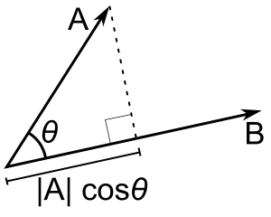
• We can interpret this scalar as a measure of the angle between the vectors.

• Formally, the dot product, in geometric terms, is:

$$ \mathbf{v} \cdot \mathbf{w} = ||\mathbf{v}|| ||\mathbf{w}||\textrm{cos}(\theta) $$

• Where $||\mathbf{v}||$ is the magnitude (length) of the vector $\mathbf{v}$. The definition it quite simple (and familiar if you recall euclidean distance):

$$ ||\mathbf{v}|| = \sqrt{v_0^2 + v_1^2 + \dots + v_n^2} $$

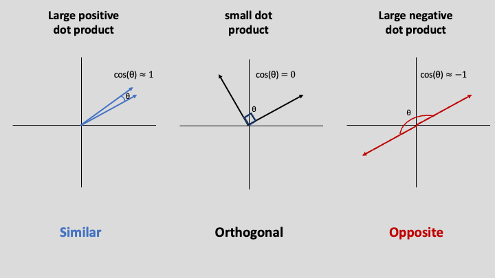
• This applet is a nice way to interactively see the relationship between magnitude, direction, and the angle between vectors via the dot product. We can visualize this relationship by noting that the dot product projects one vector onto the other (which we will make use of later with SVMs):

Recalling the properties of the cosine function, it is easy to see that the dot product between two perpendicular vectors is 0, and the dot product between two vectors which face the same direction is $|\mathbf{v}| |\mathbf{w}|$. In other words, the dot product grows as the vectors are more aligned in space.

• We can now represent our model more succiently using vectors as

  $$ y = \mathbf{w} \cdot \mathbf{x} + b $$

• We can make this even more succient by add the bias to our weight vector and adding a $1$ to the bottom of our input vector

  $$ y = \mathbf{w} \cdot \mathbf{x} $$

with $\mathbf{w}$ as

$$ \mathbf{w} = \left[\begin{array}{c} w_1 \\ w_2 \\ w_3 \\ \dots \\ w_n \\ b \end{array}\right] $$

and $\mathbf{x}$ as

$$ \mathbf{x} = \left[\begin{array}{c} x_1 \\ x_2 \\ x_3 \\ \dots \\ x_n \\ 1 \end{array}\right] $$

• Finally, we should consider how to represent many samples of many dimensions.
• To represent this, we will use matrices
• Matrices are two dimensional arrays of scalars, e.g.,

$$ \mathbf{A} = \left(\begin{array}{ccc} a_{(0,0)} & a_{(0,1)} & a_{(0,2)}\\ a_{(1,0)} & a_{(1,1)} & a_{(1,2)}\\ \end{array}\right) $$

• Note, we represent them with bolded capital letters
• $\mathbf{A}$ has two rows and three columns ($\mathbf{A}$ is a $2 \times 3$ matrix), so $a_{(1,2)}$ picks out the element in the second row and third column of $\mathbf{A}$
• In ML we tend to use rows to represent samples (usually referred to with $m$) and columns to represent features (usually referred to with $n$)
• So we can translate our n-dimensional samples into a matrix like the following

$$ \mathbf{X} = \left(\begin{array}{ccccc} a_0^{(1)} & a_1^{(1)} & a_2^{(1)} & \dots & a_n^{(1)} \\ a_0^{(2)} & a_1^{(2)} & a_2^{(2)} & \dots & a_n^{(2)} \\ \dots & \dots & \dots & \dots & \dots\\ a_n^{(m)} & a_1^{(m)} & a_2^{(m)} & \dots & a_n^{(m)} \\ \end{array}\right) $$

• We need some way of applying or parameters to these samples
• Luckily we have matrix multiplication
• Recall,

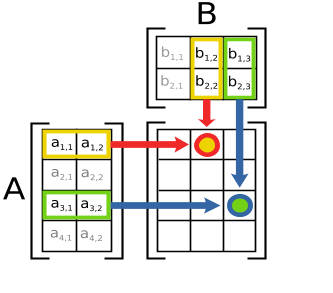
• Matrix multiplication builds on the dot product as a means of multiplying matrices together (see this video series for a refersher on matrix multiplication).

• Formally, suppose we have two matrices:

$$ \mathbf{A} = \left(\begin{array}{ccc} a_{(0,0)} & a_{(0,1)} & a_{(0,2)}\\ a_{(1,0)} & a_{(1,1)} & a_{(1,2)}\\ a_{(2,0)} & a_{(2,1)} & a_{(2,2)}\\ \end{array}\right) \hspace{1em} \textrm{and} \hspace{1em} \mathbf{B} = \left(\begin{array}{ccc} b_{(0,0)} & b_{(0,1)} & b_{(0,2)}\\ b_{(1,0)} & b_{(1,1)} & b_{(1,2)}\\ b_{(2,0)} & b_{(2,1)} & b_{(2,2)}\\ \end{array}\right) $$

• Matrix multiplication would return a new matrix:

$$ \mathbf{C} = \left(\begin{array}{ccc} c_{(0,0)} & c_{(0,1)} & c_{(0,2)}\\ c_{(1,0)} & c_{(1,1)} & c_{(1,2)}\\ c_{(2,0)} & c_{(2,1)} & c_{(2,2)}\\ \end{array}\right) $$

where:

$$ \begin{aligned} c_{(i,j)} &= \sum_{k=0}^{2} a_{(i,k)} b_{(k,j)} \\ &= a_{(i, 0)} b_{(0,j)} + a_{(i, 1)} b_{(1,j)} + a_{(i, 2)} b_{(2,j)} \end{aligned} $$

• Matrix multiplication has a shape restriction.

• To multiply two matrices $\mathbf{A}$ and $\mathbf{B}$, the shape of $\mathbf{A}$ must be n X m and the shape of $\mathbf{B}$ must be m X k. That is, the inner dimensions must align.

• Notice, that matrix multiplication is nothing more than the dot product between the rows in $\mathbf{A}$ and the columns in $\mathbf{B}$. So we can use matrix multiplication as a way of doing many dot products between vectors.

• We might try to straightrowardly extend our equation as follows:

  $$ y = \mathbf{w} \mathbf{X} $$

• Note, we will treat our parameters as a $n \times 1$ matrix (one weight for each feature, sharing the weights across all the samples)

• Question: Do you notice an issue here? What shape does $\mathbf{X}$ have?

• Answer: $\mathbf{X}$ is a $m \times n$ matrix (with $m$ samples of $n$ features), therefore the dimensions do not match

• We have two ways to resolve this, one is moving the $\mathbf{w}$ to the other side of $\mathbf{X}$

  $$ y = \mathbf{X} \mathbf{w} $$

• The other is swapping the dimensions of $\mathbf{X}$ using transpose:

$$ y = \mathbf{w} \mathbf{X}^\mathsf{T} $$

Cost (Loss) Function (or how we measure performance)

Question: Which is better and why?

• How do we know if our model is good?

• One natural option is to say that a line is a good fit to our data if it is as close as possible to our data

  • That is, we will consider are predictions $\mathbf{\hat{y}}$ and our true labels $\mathbf{y}$

• How close were we with each prediction?

  • $y^{(i)} - \hat{y}^{(i)}$

• We need some way of aggregating over all our predictions, one good option is the mean:

  • $ \frac{1}{m} \sum_{i=0}^{m} y^{(i)} - \hat{y}^{(i)} $ where $m$ is our number of samples

• What if we sometimes overpredict (yielding a negative difference) and sometimes underpredict (yielding a positive difference)?

  • These values would cancel out!

• We care about our average error, let's remove the sign with absolute values.

• That yields Mean Absolute Error (MSE) which is a well known cost function

$$ \textrm{MAE} := \frac{1}{m} \sum_{i=0}^{m} | y^{(i)} - \hat{y}^{(i)} | $$

• One final wrinkle concerns smoothness
• MAE is not smooth and easily differentiable
• For many optimization strategies we benefit from smooth, differential functions
• As an alternative, the standard loss function used in regression is Mean-Squared Error (MSE)

$$ \textrm{MSE} := \frac{1}{m} \sum_{i=0}^{m} (y^{(i)} - \hat{y}^{(i)} )^2$$

• Question: As cost functions, what is the main difference (empirically) between MAE and MSE?

Answer:

• Consider a sample, whose true label is 10 and for which the model predicts 14

• MAE for this sample is 4 while for MSE is 16

• Consider another sample, whose true label is 10 and for which the model predicts 20

• MAE for this sample is 10 while for MSE is 100

• As the size of the error increases

• The quadratic nature of MSE means that as errors increase linearly, the cost grows much more rapidly than with MAE

• MSE is more agressive for large errors

• A consequence could be faster convergence (given some other assumptions)

• But also a greater influence of extreme outliers. Why?

Optimization (or how to learn)

• Learning is (often) about optimization

• A best fit in linear regression is parameters that minimze the cost associated with the model

• That is, the aim is to determine the parameters which minimize MSE (yielding a line closest to the points)

• First let's formalize this point by combining the equation for linear regression with MSE:

$$ \begin{align} \underset{\mathbf{w} \in \mathbb{R}^n}{\textrm{arg min }}\textrm{MSE}(\mathbf{X}, \mathbf{y}; \mathbf{w}) &= \frac{1}{m} \sum_{i=0}^{m} (y^{(i)} - \hat{y}^{(i)} )^2 \\ &= \frac{1}{m} \sum_{i=0}^{m} (y^{(i)} - \mathbf{w}^\mathsf{T} \mathbf{x}^{(i)} )^2 \\ \end{align} $$

• Note that MSE takes as input our input and output and is parameterized (denoted with ;) by our parameters $\mathbf{w}$

Closed form (math)

• Unlike most ML models, linear regression has a analytic solution
• We can find the minimum by finding where the derivative of our loss function is 0 (recall standard optimization techniques from calculus)
• First, let's consider reformulating MSE over all of our samples

$$ \underset{\mathbf{w} \in \mathbb{R}^n}{\textrm{arg min }}\textrm{MSE}(X, y; \mathbf{w}) = \frac{1}{m} \| \mathbf{y} - \mathbf{X}\mathbf{w} \|^2 $$

• Notice the use of the vector norm, $\| \mathbf{v} \|$, which is defined as:

  $$ \| \mathbf{v} \| = \sqrt{\sum_{i=1}^{n} v_i^2} $$

• It should be easy to see how squaring the norm gets us back to our MSE

• Let's find the minimum (notice we reorder some terms to make it slightly easier)

$$ \begin{align} \partial_{\mathbf{w}} \frac{1}{m} \| \mathbf{X}\mathbf{w} - \mathbf{y} \|^2 &= 0\\ \frac{2}{m} \mathbf{X}^\mathsf{T}(\mathbf{X}\mathbf{w} - \mathbf{y}) &= 0\\ \mathbf{X}^\mathsf{T}\mathbf{X}\mathbf{w} &= \mathbf{X}^\mathsf{T} \mathbf{y} \\ \mathbf{w} &= (\mathbf{X}^\mathsf{T}\mathbf{X})^{-1}\mathbf{X}^\mathsf{T}\mathbf{y} \\ \end{align} $$

Gradient descent (dante's other inferno)

• A more general approach to optimization is gradient descent

• General Scheme:

  • Use a (twice) differentiable objective
  • Input initial guess for parameters
  • While not converged:
    1. Pick direction
    2. Increment weights in the desired direction
    3. If changes in weights/loss are under some threshold, then converged

• Let's walk through this with a single point with a single dimension

• Gradient descent one example at a time is called stochastic gradient descent

• First let's plot our cost function so we can visualize what we are trying to do

• Recalling our cost function for a point is

  $$ \textrm{MSE} := \frac{1}{m} \sum_{i=0}^{m} (w_1 x_1^{(i)} + b - y)^2$$

• And our data look like the following

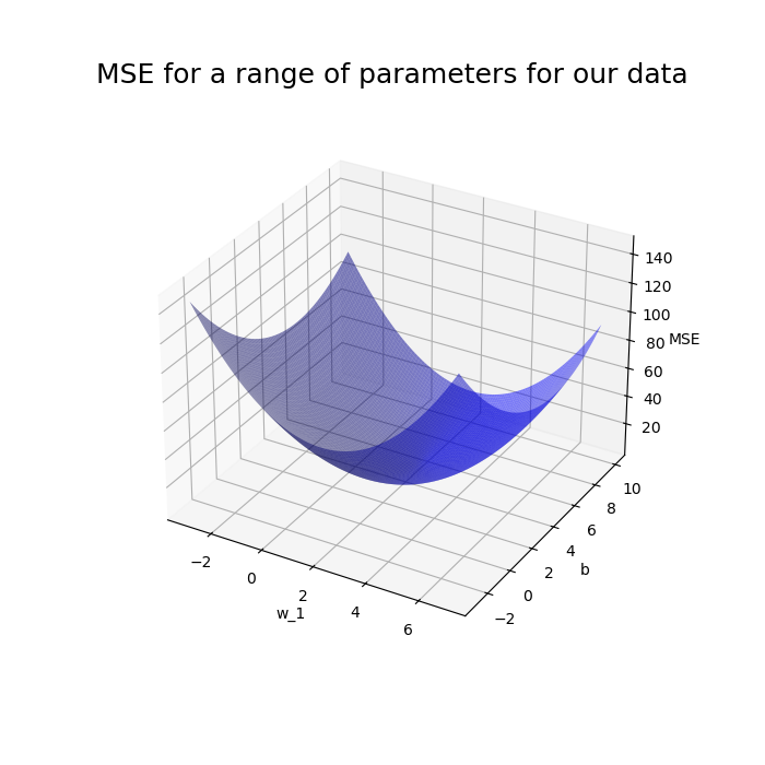
• We see that our cost function has a minimum
• The parameters for this minimum are the goal of learning
• Using our scheme we start by randomly selecting a $w_1$ and a $b$
• Let's say we selected $-2$ for $w_1$ and $10$ for $b$
• Question: Which direction do we want to move for each of these parameters? Why?

Answer:

• We want to make $w_1$ more positive and $b$ more negative
• Why: because we see the 'basin' in the plot is in that direction

• Consider the following graphic to illustrate our aims:

• We can determine this direction analytically by observing the direction of the gradient at our point
  • We consider the partial derivatives for each parameter in fact
• What's left is to determine how we should change our weights once we've selected a direction
• A standard way takes into acount the magnitude of the gradient
  • That is larger slopes mean we have 'further' to go while smaller ones mean we are near

$\theta^{\textrm{next step}} = \theta - \eta \nabla_\theta \textrm{Cost}(\mathbf{X}; \theta)$

• $\theta$ is a relevant parameter

• $\theta^{\textrm{next step}}$ is the updated parameters

• $\eta$ is the learning rate (which scales the updates)

• $\nabla_\theta$ is the gradient vector (vector of partial derivatives) with respect to parameters $\theta$

• $\textrm{Cost}(\mathbf{X}; \theta)$ is our cost function parameterized by $\theta$

• Question: What properties of a loss function would be problematic for gradient descent?

Answer:

• Non-convex functions will have local minima that will make it a challenge to know if the basin we are in is truly the optimal location

• The gradient for MSE can be adapted from our closed from solution discussion:

$$ \frac{\partial \textrm{MSE}}{\partial w_1} = 2x_1(w_1 x_1 + b - y)$$

$$ \frac{\partial \textrm{MSE}}{\partial b} = 2(w_1 x_1 + b - y)$$